A quick tutorial
This notebook provides a brief tutorial to modelling vehicle routing problems with PyVRP, introducing some of its most important modelling features. We will first solve a capacitated VRP, introducing the modelling interface and the most basic components. We then solve a VRP with time windows, where we introduce the support PyVRP has for problems with time constraints. Finally, we solve a multi-depot VRP with time windows, to showcase some additional features.
Capacitated VRP
We will first model and solve the small capacitated VRP instance with 16 clients defined in the OR-Tools documentation. This instance has an optimal solution of cost 6208. The data are as follows:
[1]:
# fmt: off
COORDS = [
    (456, 320),  # location 0 - the depot
    (228, 0),    # location 1
    (912, 0),    # location 2
    (0, 80),     # location 3
    (114, 80),   # location 4
    (570, 160),  # location 5
    (798, 160),  # location 6
    (342, 240),  # location 7
    (684, 240),  # location 8
    (570, 400),  # location 9
    (912, 400),  # location 10
    (114, 480),  # location 11
    (228, 480),  # location 12
    (342, 560),  # location 13
    (684, 560),  # location 14
    (0, 640),    # location 15
    (798, 640),  # location 16
]
DEMANDS = [0, 1, 1, 2, 4, 2, 4, 8, 8, 1, 2, 1, 2, 4, 4, 8, 8]
# fmt: on
We can use the pyvrp.Model interface to conveniently specify our vehicle routing problem using this data. A full description of the Model interface is given in our API documentation.
[2]:
from pyvrp import Model

m = Model()
m.add_vehicle_type(4, capacity=15)
depot = m.add_depot(x=COORDS[0][0], y=COORDS[0][1])
clients = [
    m.add_client(x=COORDS[idx][0], y=COORDS[idx][1], demand=DEMANDS[idx])
    for idx in range(1, len(COORDS))
]

locations = [depot, *clients]
for frm in locations:
    for to in locations:
        distance = abs(frm.x - to.x) + abs(frm.y - to.y)  # Manhattan
        m.add_edge(frm, to, distance=distance)
Let’s inspect the resulting data instance.
[3]:
import matplotlib.pyplot as plt

from pyvrp.plotting import plot_coordinates

_, ax = plt.subplots(figsize=(8, 8))
plot_coordinates(m.data(), ax=ax)
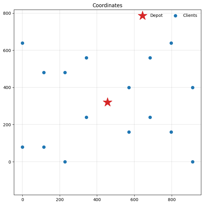
The instance looks good, so we are ready to solve it. Let’s do so with a second of runtime.
[4]:
from pyvrp.stop import MaxRuntime

res = m.solve(stop=MaxRuntime(1))  # one second
print(res)
Solution results
================
    # routes: 4
   # clients: 16
   objective: 6208.00
# iterations: 1420
    run-time: 1.00 seconds

Routes
------
Route #1: 12 11 15 13
Route #2: 8 6 2 5
Route #3: 9 10 16 14
Route #4: 1 4 3 7
Good! Our solution attains the same objective value as the optimal solution OR-Tools finds. Let’s inspect our solution more closely.
[5]:
from pyvrp.plotting import plot_solution

_, ax = plt.subplots(figsize=(8, 8))
plot_solution(res.best, m.data(), ax=ax)
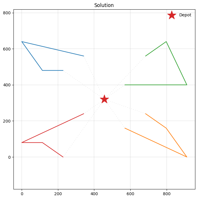
We have just solved our first vehicle routing problem using PyVRP!
VRP with time windows
Besides the capacitated VRP, PyVRP also supports the VRP with time windows. Let’s see if we can also solve such an instance, again following the OR-Tools documentation. Like in the OR-Tools example, we will ignore capacity restrictions, and give each vehicle a maximum route duration of 30. Unlike the OR-Tools example, we still aim to minimise the total travel distance, not duration.
[6]:
# fmt: off
DURATION_MATRIX = [
        [0, 6, 9, 8, 7, 3, 6, 2, 3, 2, 6, 6, 4, 4, 5, 9, 7],
        [6, 0, 8, 3, 2, 6, 8, 4, 8, 8, 13, 7, 5, 8, 12, 10, 14],
        [9, 8, 0, 11, 10, 6, 3, 9, 5, 8, 4, 15, 14, 13, 9, 18, 9],
        [8, 3, 11, 0, 1, 7, 10, 6, 10, 10, 14, 6, 7, 9, 14, 6, 16],
        [7, 2, 10, 1, 0, 6, 9, 4, 8, 9, 13, 4, 6, 8, 12, 8, 14],
        [3, 6, 6, 7, 6, 0, 2, 3, 2, 2, 7, 9, 7, 7, 6, 12, 8],
        [6, 8, 3, 10, 9, 2, 0, 6, 2, 5, 4, 12, 10, 10, 6, 15, 5],
        [2, 4, 9, 6, 4, 3, 6, 0, 4, 4, 8, 5, 4, 3, 7, 8, 10],
        [3, 8, 5, 10, 8, 2, 2, 4, 0, 3, 4, 9, 8, 7, 3, 13, 6],
        [2, 8, 8, 10, 9, 2, 5, 4, 3, 0, 4, 6, 5, 4, 3, 9, 5],
        [6, 13, 4, 14, 13, 7, 4, 8, 4, 4, 0, 10, 9, 8, 4, 13, 4],
        [6, 7, 15, 6, 4, 9, 12, 5, 9, 6, 10, 0, 1, 3, 7, 3, 10],
        [4, 5, 14, 7, 6, 7, 10, 4, 8, 5, 9, 1, 0, 2, 6, 4, 8],
        [4, 8, 13, 9, 8, 7, 10, 3, 7, 4, 8, 3, 2, 0, 4, 5, 6],
        [5, 12, 9, 14, 12, 6, 6, 7, 3, 3, 4, 7, 6, 4, 0, 9, 2],
        [9, 10, 18, 6, 8, 12, 15, 8, 13, 9, 13, 3, 4, 5, 9, 0, 9],
        [7, 14, 9, 16, 14, 8, 5, 10, 6, 5, 4, 10, 8, 6, 2, 9, 0],
]
TIME_WINDOWS = [
        (0, 999),  # location 0 - the depot (modified to be unrestricted)
        (7, 12),   # location 1
        (10, 15),  # location 2
        (16, 18),  # location 3
        (10, 13),  # location 4
        (0, 5),    # location 5
        (5, 10),   # location 6
        (0, 4),    # location 7
        (5, 10),   # location 8
        (0, 3),    # location 9
        (10, 16),  # location 10
        (10, 15),  # location 11
        (0, 5),    # location 12
        (5, 10),   # location 13
        (7, 8),    # location 14
        (10, 15),  # location 15
        (11, 15),  # location 16
]
# fmt: on
We now need to specify the time windows for all locations, and the duration of travelling along each edge.
[7]:
m = Model()
m.add_vehicle_type(4, max_duration=30)
depot = m.add_depot(
    x=COORDS[0][0],
    y=COORDS[0][1],
    tw_early=TIME_WINDOWS[0][0],
    tw_late=TIME_WINDOWS[0][1],
)
clients = [
    m.add_client(
        x=COORDS[idx][0],
        y=COORDS[idx][1],
        tw_early=TIME_WINDOWS[idx][0],
        tw_late=TIME_WINDOWS[idx][1],
    )
    for idx in range(1, len(COORDS))
]

locations = [depot, *clients]
for frm_idx, frm in enumerate(locations):
    for to_idx, to in enumerate(locations):
        distance = abs(frm.x - to.x) + abs(frm.y - to.y)  # Manhattan
        duration = DURATION_MATRIX[frm_idx][to_idx]
        m.add_edge(frm, to, distance=distance, duration=duration)
[8]:
res = m.solve(stop=MaxRuntime(1))  # one second
print(res)
Solution results
================
    # routes: 4
   # clients: 16
   objective: 6528.00
# iterations: 1078
    run-time: 1.00 seconds

Routes
------
Route #1: 9 14 16
Route #2: 7 1 4 3
Route #3: 5 8 6 2 10
Route #4: 12 13 15 11
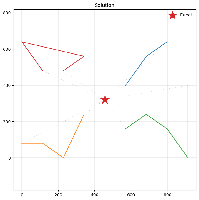
Due to the hard time windows requirements, the total travel distance has increased slightly compared to our solution for the capacitated VRP. Let’s have a look at the new solution.
[9]:
_, ax = plt.subplots(figsize=(8, 8))
plot_solution(res.best, m.data(), ax=ax)
Multi-depot VRP with time windows
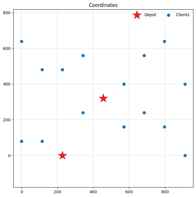
Let’s now solve a VRP with multiple depots and time windows. We consider two depots, and two vehicles per depot that have to start and end their routes at their respective depot. For this, we will re-use some of the data from the VRPTW case, but change the time window data slightly: the first client now becomes the second depot.
[10]:
# fmt: off
TIME_WINDOWS = [
    (0, 999),  # location 0 - a depot (modified to be unrestricted)
    (0, 999),  # location 1 - a depot (modified to be unrestricted)
    (10, 15),  # location 2
    (16, 18),  # location 3
    (10, 13),  # location 4
    (0, 5),    # location 5
    (5, 10),   # location 6
    (0, 4),    # location 7
    (5, 10),   # location 8
    (0, 3),    # location 9
    (10, 16),  # location 10
    (10, 15),  # location 11
    (0, 5),    # location 12
    (5, 10),   # location 13
    (7, 8),    # location 14
    (10, 15),  # location 15
    (11, 15),  # location 16
]
# fmt: on
[11]:
m = Model()
depots = [
    m.add_depot(
        x=COORDS[idx][0],
        y=COORDS[idx][1],
        tw_early=TIME_WINDOWS[idx][0],
        tw_late=TIME_WINDOWS[idx][1],
    )
    for idx in range(2)
]

for depot in depots:
    # Two vehicles at each of the depots, with maximum route durations
    # of 30.
    m.add_vehicle_type(2, depot=depot, max_duration=30)

clients = [
    m.add_client(
        x=COORDS[idx][0],
        y=COORDS[idx][1],
        tw_early=TIME_WINDOWS[idx][0],
        tw_late=TIME_WINDOWS[idx][1],
    )
    for idx in range(2, len(COORDS))
]

locations = [*depots, *clients]
for frm_idx, frm in enumerate(locations):
    for to_idx, to in enumerate(locations):
        distance = abs(frm.x - to.x) + abs(frm.y - to.y)  # Manhattan
        duration = DURATION_MATRIX[frm_idx][to_idx]
        m.add_edge(frm, to, distance=distance, duration=duration)
Let’s have a look at the modified data instance to familiarise ourself with the changes.
[12]:
_, ax = plt.subplots(figsize=(8, 8))
plot_coordinates(m.data(), ax=ax)
Let’s solve the instance.
[13]:
res = m.solve(stop=MaxRuntime(1))  # one second
print(res)
Solution results
================
    # routes: 4
   # clients: 15
   objective: 6004.00
# iterations: 1213
    run-time: 1.00 seconds

Routes
------
Route #1: 9 14 16
Route #2: 7 5 8 6 2 10
Route #3: 12 13 15 11
Route #4: 4 3
[14]:
_, ax = plt.subplots(figsize=(8, 8))
plot_solution(res.best, m.data(), ax=ax)
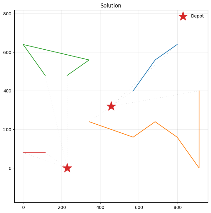
This concludes the brief tutorial: you now know how to model and solve VRP problems using PyVRP’s Model interface. PyVRP supports several additional VRP variants we have not covered here. Have a look at the VRP introduction and other documentation pages to see how those can be modelled and solved.