Vehicle Routing Problem with Time Windows

This notebook shows how to use the PyVRP library to solve the Vehicle Routing Problem with Time Windows (VRPTW).

A VRPTW instance is defined on a complete graph \(G=(V,A)\), where \(V\) is the vertex set and \(A\) is the arc set. The vertex set \(V\) is partitioned into \(V=\{0\} \cup V_c\), where \(0\) represents the depot and \(V_c=\{1, \dots, n\}\) denotes the set of \(n\) customers. Each arc \((i, j) \in A\) has a weight \(d_{ij} \ge 0\) that represents the travel distance from \(i \in V\) to \(j \in V\), which need not to be symmetric and/or euclidean. Each customer \(i \in V_c\) has a demand \(q_{i} \ge 0\), a service time \(s_{i} \ge 0\) and a (hard) time window \(\left[e_i, l_i\right]\) that denotes the earliest and latest time that service can start. A vehicle is allowed to arrive at a customer location before the beginning of the time window, but it must wait for the window to open to start the delivery. Each vehicle must return to the depot before the end of the depot time window \(H\). We assume that there is an unlimited number of homogeneous vehicles available, each with maximum capacity \(Q > 0\).

A feasible solution to the VRPTW consists of a set of routes that all begin and end at the depot, such that each customer is visited exactly once, all customers are served within their time windows and none of the vehicles exceed their capacity. The objective is to find a feasible solution that minimizes the total distance.

In the following, we will show how to configure the Hybrid Genetic Search algorithm to solve three different VRPTW instances. Moreover, we demonstrate how to use plotting and diagnostics utilities from the PyVRP library to analyze the results.

Basic example

We’ll start with a basic example that loads an instance and solves it using a standard configuration. First, let’s import some necessary components.

[1]:

from typing import Dict, Optional
from pathlib import Path
from IPython.display import display

import matplotlib.pyplot as plt
import pandas as pd
import vrplib

from pyvrp import (
    GeneticAlgorithm,
    GeneticAlgorithmParams,
    Individual,
    PenaltyManager,
    Population,
    PopulationParams,
    ProblemData,
    Result,
    XorShift128,
    diagnostics,
    plotting,
    read,
)
from pyvrp.crossover import selective_route_exchange as srex
from pyvrp.diversity import broken_pairs_distance as bpd
from pyvrp.educate import (
    NODE_OPERATORS,
    ROUTE_OPERATORS,
    LocalSearch,
    compute_neighbours,
)
from pyvrp.stop import MaxIterations, MaxRuntime, StoppingCriterion

Read and plot instance

We will first load one of the classical Solomon instances. We use the function pyvrp.read, which reads the instance file and converts it to a ProblemData instance. We pass the following arguments:

instance_format='solomon': this parses the instance file as a Solomon formatted instance (as opposed to VRPLIB formatted instances),
round_func='trunc1': this compute distances with 1 decimal precision, by multipliying all distances by 10 and converting to integers (i.e., following the DIMACS VRP challenge convention).

[2]:

instance = read(
    "data/RC208.vrp", instance_format="solomon", round_func="trunc1"
)
instance_bks = vrplib.read_solution("data/RC208.sol")

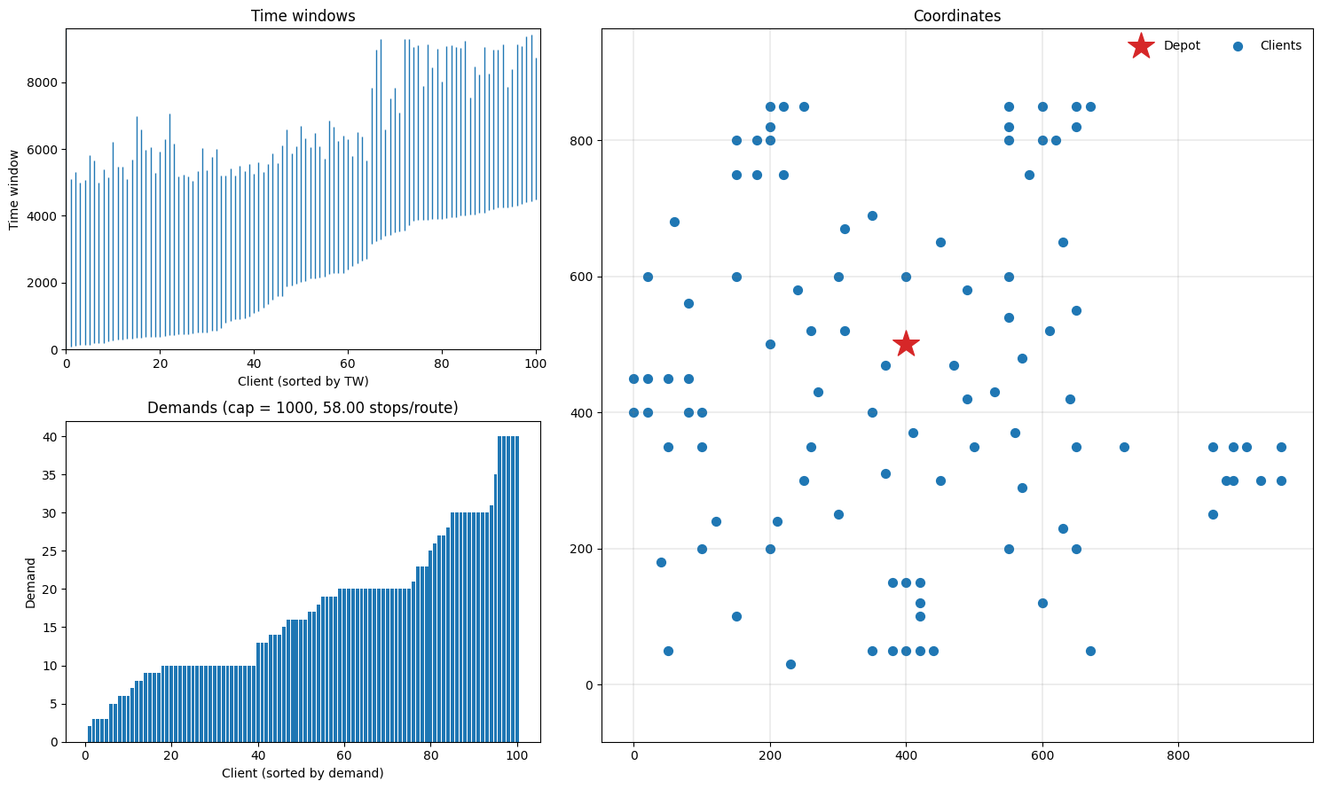
Let’s plot the instance and see what we have. The function plotting.plot_instance will plot time windows, demands and coordinates, which should give us a good impression of what the instance looks like (note that these can also be plotted separately using the plotting.plot_* functions.

[3]:

fig = plt.figure(figsize=(15, 9))
plotting.plot_instance(instance, fig)

Configuring Hybrid Genetic Search

Now we will implement the solve function that sets up the necessary components of the Hybrid Genetic Search algorithm, which is a hybrid between a genetic algorithm and local search. The components include Population, LocalSearch, and the PenaltyManager. Then we will create the GeneticAlgorithm object and run it until our desired StoppingCriterion is met.

[4]:

def solve(
    data: ProblemData,
    seed: int,
    max_runtime: Optional[float] = None,
    max_iterations: Optional[int] = None,
    **kwargs,
):
    rng = XorShift128(seed=seed)
    pen_manager = PenaltyManager()
    pop_params = PopulationParams()
    pop = Population(bpd, params=pop_params)
    ls = LocalSearch(data, rng, compute_neighbours(data))

    for op in NODE_OPERATORS:
        ls.add_node_operator(op(data))

    for op in ROUTE_OPERATORS:
        ls.add_route_operator(op(data))

    init = [
        Individual.make_random(data, rng)
        for _ in range(pop_params.min_pop_size)
    ]
    ga_params = GeneticAlgorithmParams(collect_statistics=True)
    algo = GeneticAlgorithm(
        data, pen_manager, rng, pop, ls, srex, init, params=ga_params
    )

    if max_runtime is not None:
        stop = MaxRuntime(max_runtime)
    else:
        assert max_iterations is not None
        stop = MaxIterations(max_iterations)

    return algo.run(stop)

Solving an instance

Now let’s run the algorithm using our solve function and compare the result with the best known solution. To compute the cost for the solution, we need a CostEvaluator instance. We can get it from the penalty manager.

[5]:

def report_gap(best_cost: float, bks: Dict, scale_factor: float = 10):
    objective = best_cost / scale_factor
    bks_cost = bks["cost"]
    pct_diff = 100 * (objective - bks_cost) / bks_cost

    print(f"Found a solution with cost: {objective}.")
    print(f"This is {pct_diff:.1f}% worse than the best known", end=" ")
    print(f"solution, which is {bks_cost}.")


cost_evaluator = PenaltyManager().get_cost_evaluator()
result = solve(instance, seed=42, max_runtime=5)
report_gap(cost_evaluator.cost(result.best), instance_bks)

Found a solution with cost: 776.1.
This is 0.0% worse than the best known solution, which is 776.1.

We’ve managed to find the best known solution in 5 seconds!

Plot results

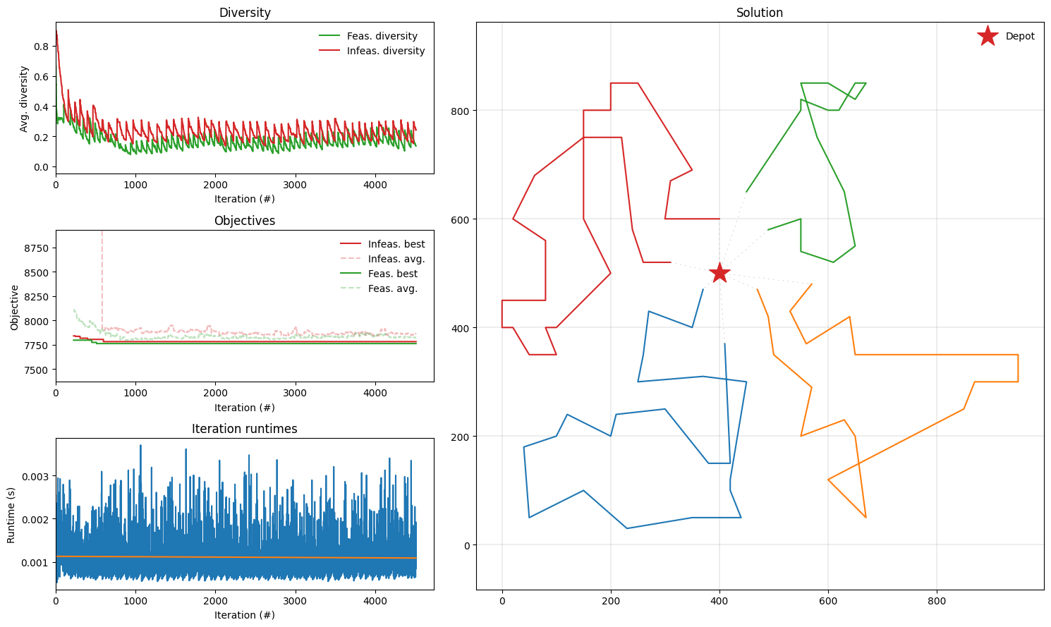
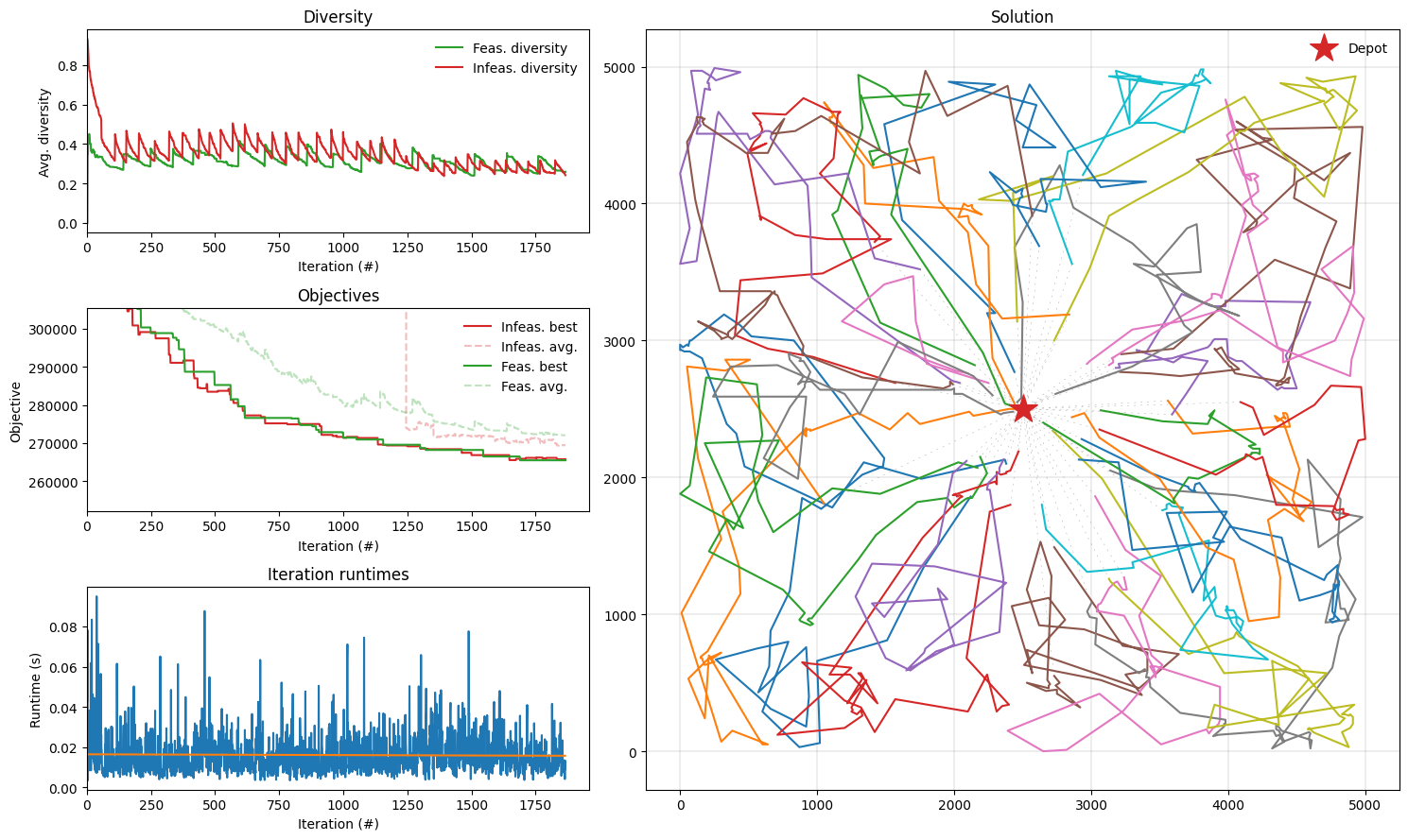
The result object (of type Result) contains useful statistics about the optimization since we set collect_statistics=True in GeneticAlgorithmParams (see the solve function). We can now plot these statistics as well as the final solution use plotting.plot_result.

[6]:

def plot_result(result: Result, instance: ProblemData):
    fig = plt.figure(figsize=(15, 9))
    plotting.plot_result(result, instance, fig)
    fig.tight_layout()


plot_result(result, instance)

Inspect routes

We can also inspect some statistics of the different routes, such as route distance and duration, number of stops and total demand, using diagnostics.get_all_route_statistics. Let’s verify that the cost of our solution is equal to the sum of the distances.

[7]:

cost_evaluator = PenaltyManager().get_cost_evaluator()
solution = result.best
route_stats = diagnostics.get_all_route_statistics(solution, instance)
route_stats_df = pd.DataFrame(route_stats)

# Verify that cost is equal to total distance
assert route_stats_df["distance"].sum() == cost_evaluator.cost(solution)

display(route_stats_df.head())

	distance	end_time	duration	wait_time	service_time	num_stops	total_demand	fillrate	is_feasible	is_empty
0	2187	7043	7043	2156	2700	27	465	0.465	True	False
1	1983	6862	6862	2479	2400	24	381	0.381	True	False
2	1325	6016	6016	2991	1700	17	286	0.286	True	False
3	2266	7295	7295	1829	3200	32	592	0.592	True	False

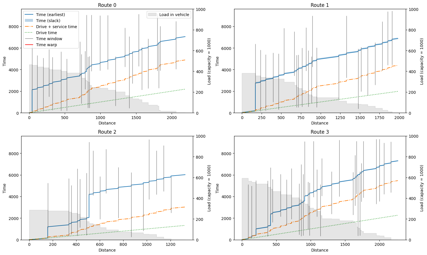
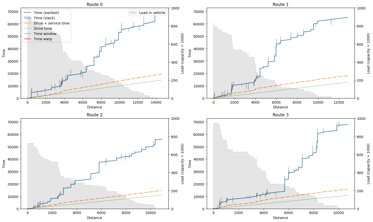
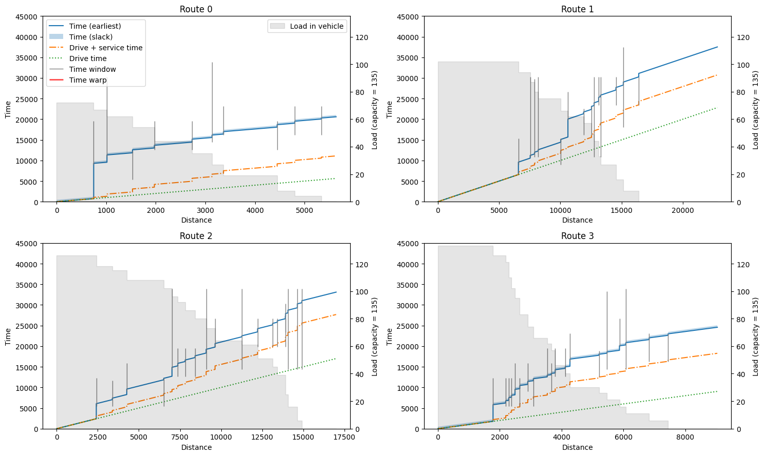
We can inspect the routes in more detail using the plotting.plot_route_schedule function. This will plot distance on the x-axis, and time on the y-axis, separating actual travel/driving time from waiting and service time. The clients visited are plotted as grey vertical bars indicating their time windows. When a vehicle arrives too early at a customer, we can see a jump to the start of the time window in the main (earliest) time line. In some cases, there is slack in the route indicated by a semi-transparent region on top of the earliest time line (see plot of Route 1). The grey background indicates the remaining load of the truck during the route, where the (right) y-axis ends at the vehicle capacity.

[8]:

def plot_route_schedule(result: Result, instance: ProblemData):
    fig, axarr = plt.subplots(2, 2, figsize=(15, 9))

    routes = result.best.get_routes()
    for idx, (ax, route) in enumerate(zip(axarr.reshape(-1), routes)):
        plotting.plot_route_schedule(
            instance, route, title=f"Route {idx}", ax=ax, legend=idx == 0
        )

    fig.tight_layout()


plot_route_schedule(result, instance)

Solving larger instances

Gehring & Homberger instance

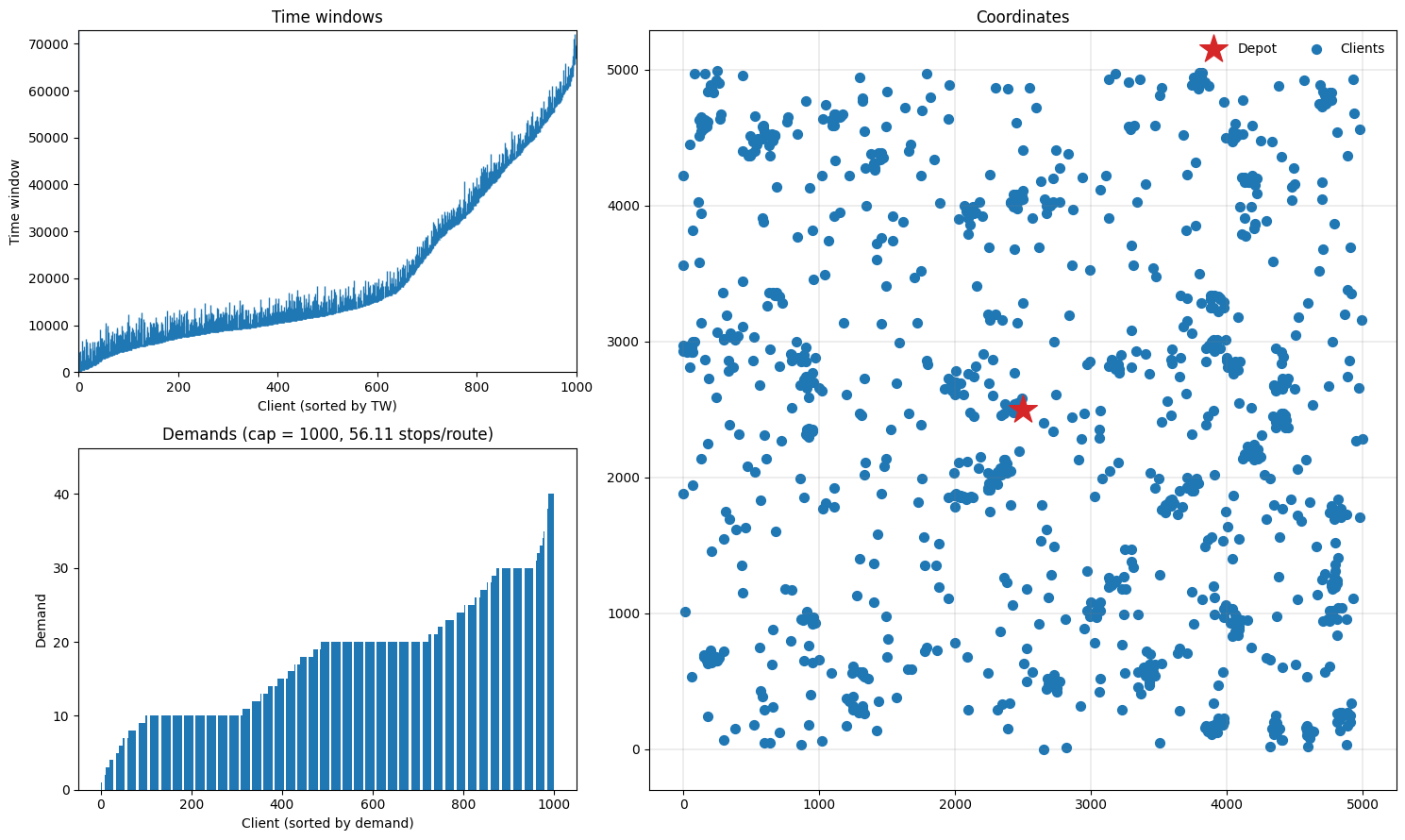
Let’s try one of the largest Gehring & Homberger instances (1000 customers), and plot the instance, results and some routes.

[9]:

instance_gh = read(
    "data/RC2_10_5.vrp", instance_format="solomon", round_func="trunc1"
)
bks_gh = vrplib.read_solution("data/RC2_10_5.sol")

fig = plt.figure(figsize=(15, 9))
plotting.plot_instance(instance_gh, fig)

result_gh = solve(instance_gh, seed=42, max_runtime=30)

cost_evaluator = PenaltyManager().get_cost_evaluator()
best_cost_gh = cost_evaluator.cost(result_gh.best)
report_gap(best_cost_gh, bks_gh)
plot_result(result_gh, instance_gh)
plot_route_schedule(result_gh, instance_gh)

Found a solution with cost: 26548.6.
This is 2.9% worse than the best known solution, which is 25797.5.

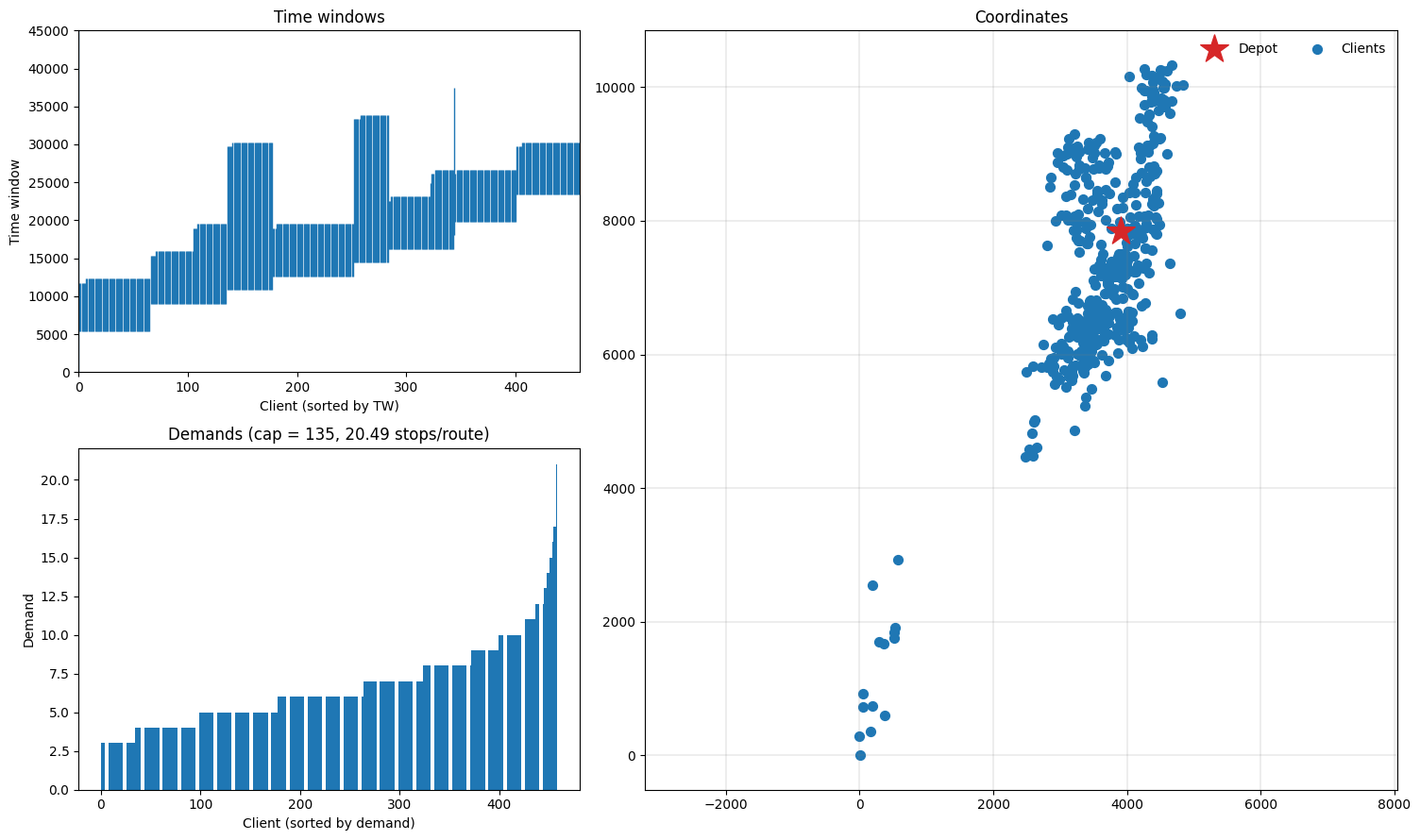
ORTEC instance (from the EURO Meets NeurIPS 2022 Competition)

Let’s also try an instance based on real data, which uses an actual over-the-road distance matrix (non-Euclidean) and atypical client distribution. Note that the file is in VRPLIB format and the distances are already integral and so there is no rounding.

[10]:

name_ortec = "ORTEC-VRPTW-ASYM-0bdff870-d1-n458-k35"
instance_ortec = read(f"data/{name_ortec}.txt")
bks_ortec = vrplib.read_solution(f"data/{name_ortec}.sol")

fig = plt.figure(figsize=(15, 9))
plotting.plot_instance(instance_ortec, fig)

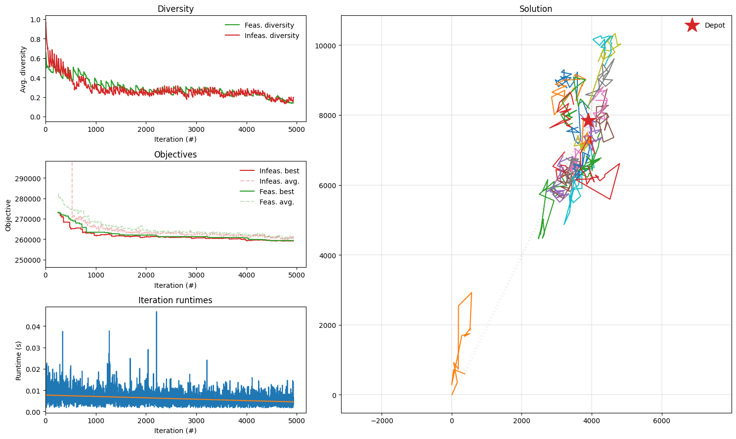
result_ortec = solve(instance_ortec, seed=42, max_runtime=30)

cost_evaluator = PenaltyManager().get_cost_evaluator()
best_cost_ortec = cost_evaluator.cost(result_ortec.best)
report_gap(best_cost_ortec, bks_ortec, scale_factor=1)
plot_result(result_ortec, instance_ortec)
plot_route_schedule(result_ortec, instance_ortec)

Found a solution with cost: 259297.0.
This is 0.2% worse than the best known solution, which is 258704.

Conclusion

In this notebook, we showed how to configure the Hybrid Genetic Search algorithm to solve the VRPTW. We run the solver on three different instances and we demonstrate how to use plotting and diagnostics utilities from the PyVRP library.